Introduction

mELO is an R implementation of DeepMind’s multidimensional Elo rating (mELO) system for evaluating agents. This package uses code directly from Alec Stephenson and Jeff Sonas’s excellent PlayerRatings package (v1.0-3, 2019-02-22).

Balduzzi, et al. (2018) proposed that a rating/evaluation method should have the following properties:

P1. Invariant: adding redundant copies of an agent or task to the data should make no difference.
P2. Continuous: the evaluation method should be robust to small changes in the data.
P3. Interpretable: hard to formalize, but the procedure should agree with intuition in basic cases.

Typical methods for performing pairwise comparisons such as Elo or Glicko violate P1 and can result in poor evaluations of agents and predictions of outcomes.

Additionally, typical methods can perform poorly in an environment where there exist cyclical or non-transitive interactions between agents or players. Below we demonstrate the utility of the mELO package with some simple examples.

Evaluating agents with non-transitive interactions

We provide some examples of how the mELO package can be used to evaluate agents and predict outcomes in the presence of non-transitive interactions. The examples are trivial but do demonstrate the weaknesses of existing methods and the utility of the mELO approach.

Rock-Paper-Scissors

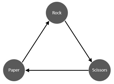
Out first model will evaluate throws in the 2-player game of Rock-Paper-Scissors. The direction of the arrows in the figure below give the winner of each thrown pair

# Load packages
library(mELO)
library(dplyr)

# Inspect data
rps_df %>% head() %>% knitr::kable()

time_index	throw_1	throw_2	outcome
1	PAPER	ROCK	1
2	ROCK	SCISSORS	1
3	SCISSORS	PAPER	1
4	ROCK	PAPER	0
5	SCISSORS	ROCK	0
6	PAPER	SCISSORS	0

The second and third columns give the throws chosen. A 1 in the outcome field denotes a win for throw 1, 0 denotes a win for throw 2. The rps_df data has 120 matches.

ELO model

The predictions probabilities estimated by an Elo model are given by \[ \hat{p}_{ij} = \sigma (\alpha(r_i + \gamma_i - r_j)) \] Where $\hat{p}_{ij}$ is the estimated probability of player $i$ beating player $j$, $r_i$ is the current rating of player $i$, $\alpha = \ln(10)/400$, $\gamma_i$ represents the first move or home ground advantage for player $i$ and \[ \sigma(x) = \frac{1}{(1+ e^{-x})}. \]

After a match at time $t$, the following rule is used to update ratings \[ r_i^{t+1} = r^t_i + \eta \delta_{ij} \] where $\eta$ is the learning rate and $\delta = \hat{p}_{ij} - y$ where $y \in \{0, 1\}$ is the outcome of the match for player $i$.

The following code fits a standard Elo model using the ELO() function with a default eta (the learning rate) and p1_advantage (Player 1 advantage i.e; first mover or home ground advantage).

# Fit model
rps_ELO <- ELO(rps_df)
# Display output
rps_ELO
#> 
#> ELO Ratings For 3 Players Playing 120 Games
#> 
#>     Player Rating Games Win Draw Loss Lag
#> 1 SCISSORS 2204.6    80  40    0   40   0
#> 2     ROCK 2204.6    80  40    0   40   1
#> 3    PAPER 2190.7    80  40    0   40   0

Now we can generate some predictions on a sample of the data and compare them to the actual outcomes

rps_ELO_preds <- predict(
    rps_ELO,
    head(rps_df)
)

results_df <- data.frame(
    head(rps_df),
    ELO_preds = rps_ELO_preds %>% round(3)
)
results_df %>% knitr::kable()

time_index	throw_1	throw_2	outcome	ELO_preds
1	PAPER	ROCK	1	0.48
2	ROCK	SCISSORS	1	0.50
3	SCISSORS	PAPER	1	0.52
4	ROCK	PAPER	0	0.52
5	SCISSORS	ROCK	0	0.50
6	PAPER	SCISSORS	0	0.48

We observe that the Elo predictions are very poor. We can plot the history of the ratings using the plot() function

plot(rps_ELO)

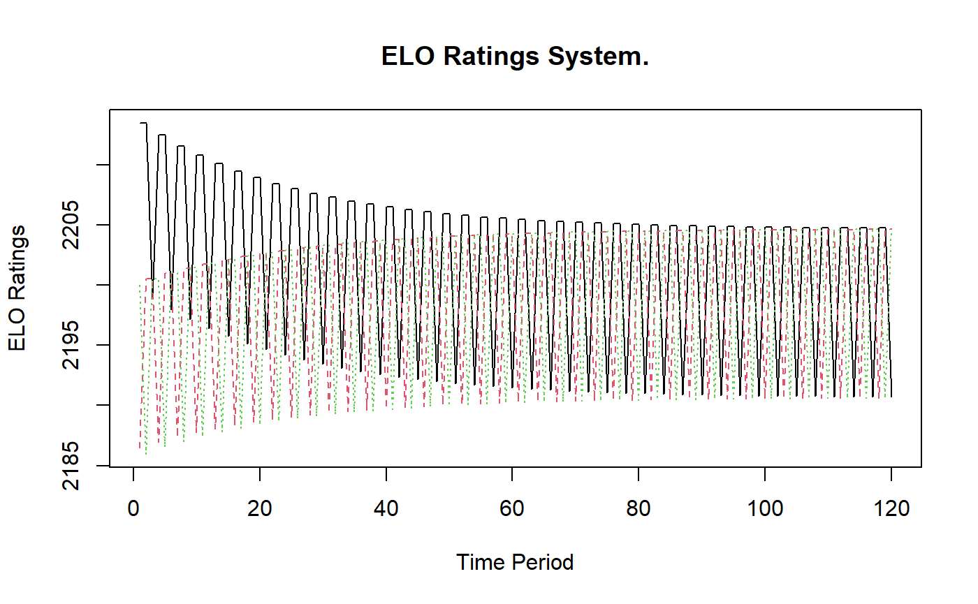
We note that the ratings bounce up and down as the throws consistently lose and win to the same players.

Because the ability of an agent is described by a single parameter, the Elo ratings bake-in the assumption that relative abilities are transitive. This assumption is clearly inappropriate in this setting (and likely many others). The Elo model completely fails to capture the dynamics of this simple game and cannot be used to adequately rate or evaluate throws or predict outcomes.

mELO model

The success probabilities estimated by an mELO model are given by \[ \hat{p}_{ij} = \sigma (\alpha(r_i + \gamma_i - r_j + \textbf{c}_i \Omega \textbf{c}_j' )) \] where $\Omega$ is a $2k \times 2k$ matrix constructed such that \[ \Omega = \sum_{i=1}^{k} (\textbf{e}_{2i-1} \textbf{e}_{2i}' - \textbf{e}_{2i} \textbf{e}_{2i-1}') \] and $\textbf{c}_i$ is a row vector of the $m \times 2k$ dimension $\textbf{C}$ matrix which encodes the non-transitive interactions between the $m$ agents or players. $\textbf{e}_j$ are standard basis vectors spanning the columns of $\Omega$. Larger $k$ allows for better estimates in situations with more complex dynamics, which we will observe later.

After a match, the following rules are used to update ratings \[ r_i^{t+1} = r^t_i + \eta_1 \delta_{ij}, \] \[ \textbf{c}_i^{t+1} = \textbf{c}^t_i + \eta_2 \delta_{ij} \Omega \textbf{c}^t_j \] where $\eta_1$ and $\eta_2$ are the learning rates for the ratings vector $\textbf{r}$ and $\textbf{C}$ matrix respectively.

The following code fits a mELO model using the mELO() function with a default $k=1$, learning rates and player 1 advantage parameters.

# Fit model
rps_mELO <- mELO(rps_df)
# Display output
rps_mELO
#> 
#> mELO Ratings For 3 Players Playing 120 Games
#> 
#> k = 1.
#> 
#>     Player Rating Games Win Draw Loss Lag
#> 1    PAPER 2211.4    80  40    0   40   0
#> 2     ROCK 2194.6    80  40    0   40   1
#> 3 SCISSORS 2193.9    80  40    0   40   0

Predictions can be generated using

rps_mELO_preds <- predict(
    rps_mELO,
    head(rps_df)
)

results_df <- data.frame(
    head(rps_df),
    mELO_preds = rps_mELO_preds %>% round(3)
)
results_df %>% knitr::kable()

time_index	throw_1	throw_2	outcome	mELO_preds
1	PAPER	ROCK	1	0.999
2	ROCK	SCISSORS	1	0.999
3	SCISSORS	PAPER	1	0.999
4	ROCK	PAPER	0	0.001
5	SCISSORS	ROCK	0	0.001
6	PAPER	SCISSORS	0	0.001

or with the model_pred_mat() helper function

model_pred_mat(
  rps_mELO,
  rps_df[[2]],
  round = 3
) %>%
  knitr::kable()

	PAPER	ROCK	SCISSORS
PAPER	0.500	0.999	0.001
ROCK	0.001	0.500	0.999
SCISSORS	0.999	0.001	0.500

We observe that the mELO predictions are very good. They accurately capture the cyclical, non-transitive properties of the game. We can plot the history of the ratings using the plot() function

plot(rps_mELO)

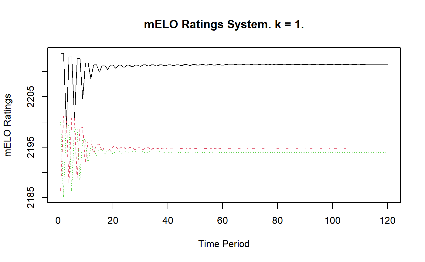
The mELO ratings quickly stabilise, but we note that the ratings aren’t all equal which we might expect for agents that exhibit perfectly cyclical dynamics. However, the ratings by themselves are not the only things that matter when making predictions from a mELO model. Let \[ \textbf{A} = \textbf{C} \Omega \textbf{C}' \] be the $m \times m$ advantage-disadvantage matrix for our model, where $a_{ij}$ is the advantage agent $i$ has over agent $j$. mELO uses elements of this matrix when making predictions. The $\textbf{A}$ matrix can be obtained from a mELO model using get_adv_mat()

get_adv_mat(rps_mELO) %>%
  round(0) %>%
  knitr::kable()

	PAPER	ROCK	SCISSORS
PAPER	0	1118	-1166
ROCK	-1118	0	1141
SCISSORS	1166	-1141	0

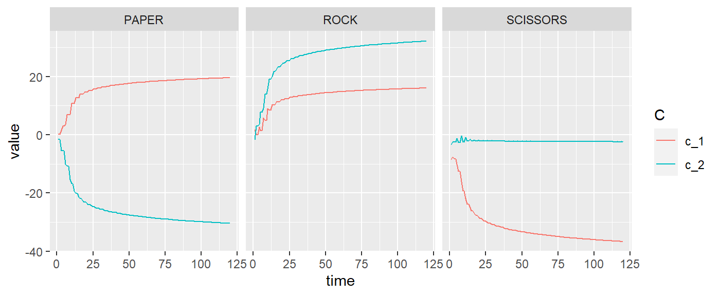
The advantage-disadvantage estimates are what result in the accurate win probabilities despite the stability and inequality of ratings. The $\textbf{C}$ matrix can be obtained with rps_mELO$c_mat and an array of its history can be obtained using rps_mELO$c_mat_history.

A function has been provided to easily plot the evolution of the $\text{c}$ vectors for each agent

plot_c_mat(rps_mELO)

Rock-Paper-Scissors-Fire-Water

In this example we will consider a more complex variant of rock-paper-scissors. Here, there are two additional throws, fire and water which behave according to the figure below

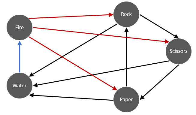
Observe that fire beats everything except water, and water loses to everything except fire.

Knowing that a regular Elo model will obviously fail to model this situation accurately, we will begin by fitting a mELO model with $k=1$

mELO model with $k=1$

rpsfw_mELO_1 <- mELO(rpsfw_df, k=1)
rpsfw_mELO_1
#> 
#> mELO Ratings For 5 Players Playing 375 Games
#> 
#> k = 1.
#> 
#>     Player Rating Games Win Draw Loss Lag
#> 1     FIRE 2371.9   150  90   30   30   2
#> 2     ROCK 2275.8   150  60   30   60   3
#> 3    PAPER 2215.7   150  60   30   60   0
#> 4 SCISSORS 2209.8   150  60   30   60   5
#> 5    WATER 1926.8   150  30   30   90   1

# Sample data to make predictions on
rpsfw_sample_df <- rpsfw_df %>%
    filter(outcome == 1) %>%
    mutate(time_index = NA) %>%
    distinct() %>%
    arrange(throw_1, throw_2) %>%
    mutate(time_index = 1:n())

# Get predictions
rpsfw_mELO_preds <- predict(
    rpsfw_mELO_1,
    rpsfw_sample_df
)
data.frame(
    rpsfw_sample_df,
    mELO_preds = rpsfw_mELO_preds %>% round(3)
)
#>    time_index  throw_1  throw_2 outcome mELO_preds
#> 1           1     FIRE    PAPER       1      1.000
#> 2           2     FIRE     ROCK       1      0.998
#> 3           3     FIRE SCISSORS       1      0.991
#> 4           4    PAPER     ROCK       1      0.057
#> 5           5    PAPER    WATER       1      0.998
#> 6           6     ROCK SCISSORS       1      0.923
#> 7           7     ROCK    WATER       1      0.935
#> 8           8 SCISSORS    PAPER       1      0.036
#> 9           9 SCISSORS    WATER       1      0.989
#> 10         10    WATER     FIRE       1      0.979

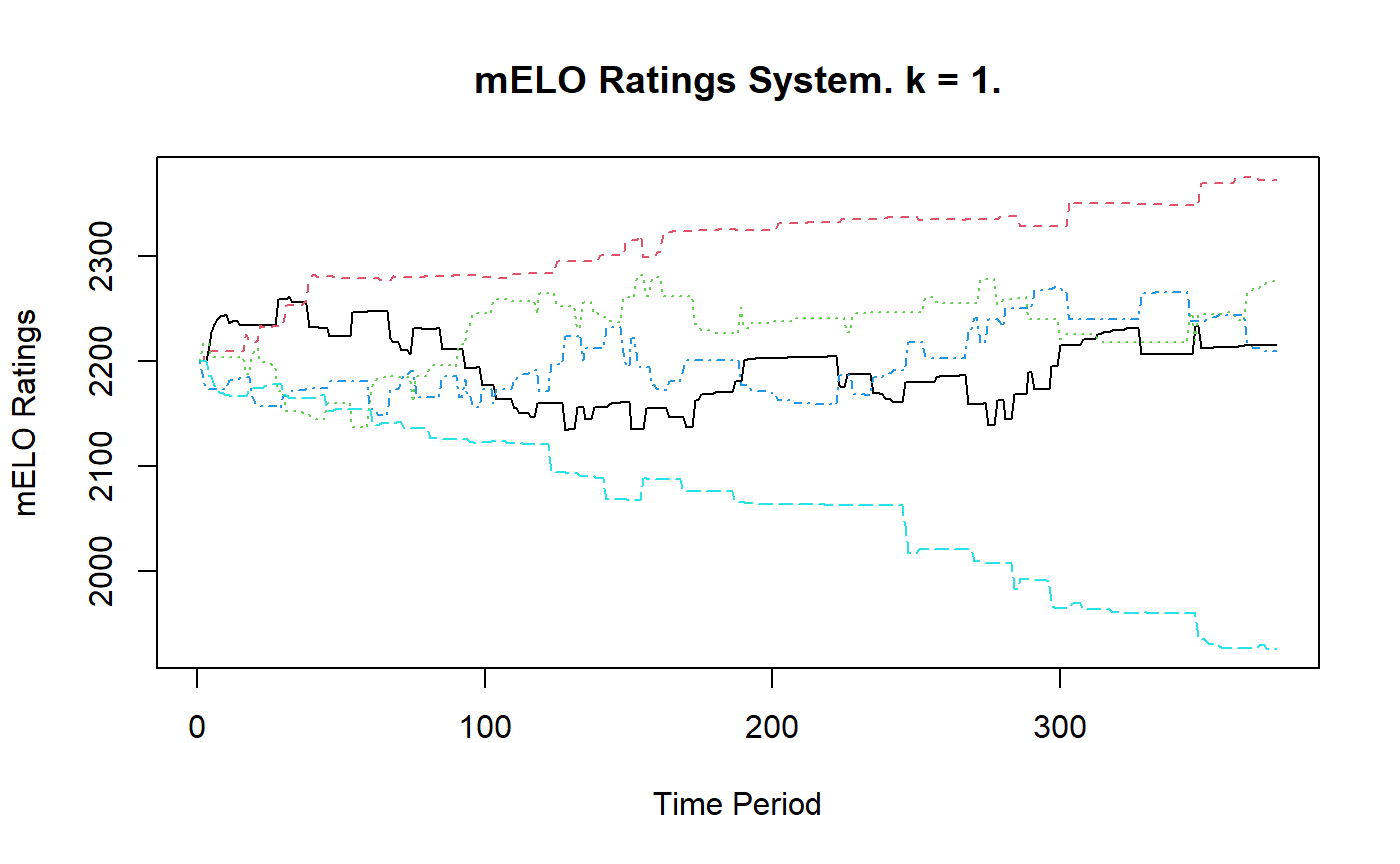
The predictions are almost right, but according to the rules, paper will always beat rock, and scissors always beat paper. Let’s look at the evolution of the ratings and the vectors

plot(rpsfw_mELO_1)

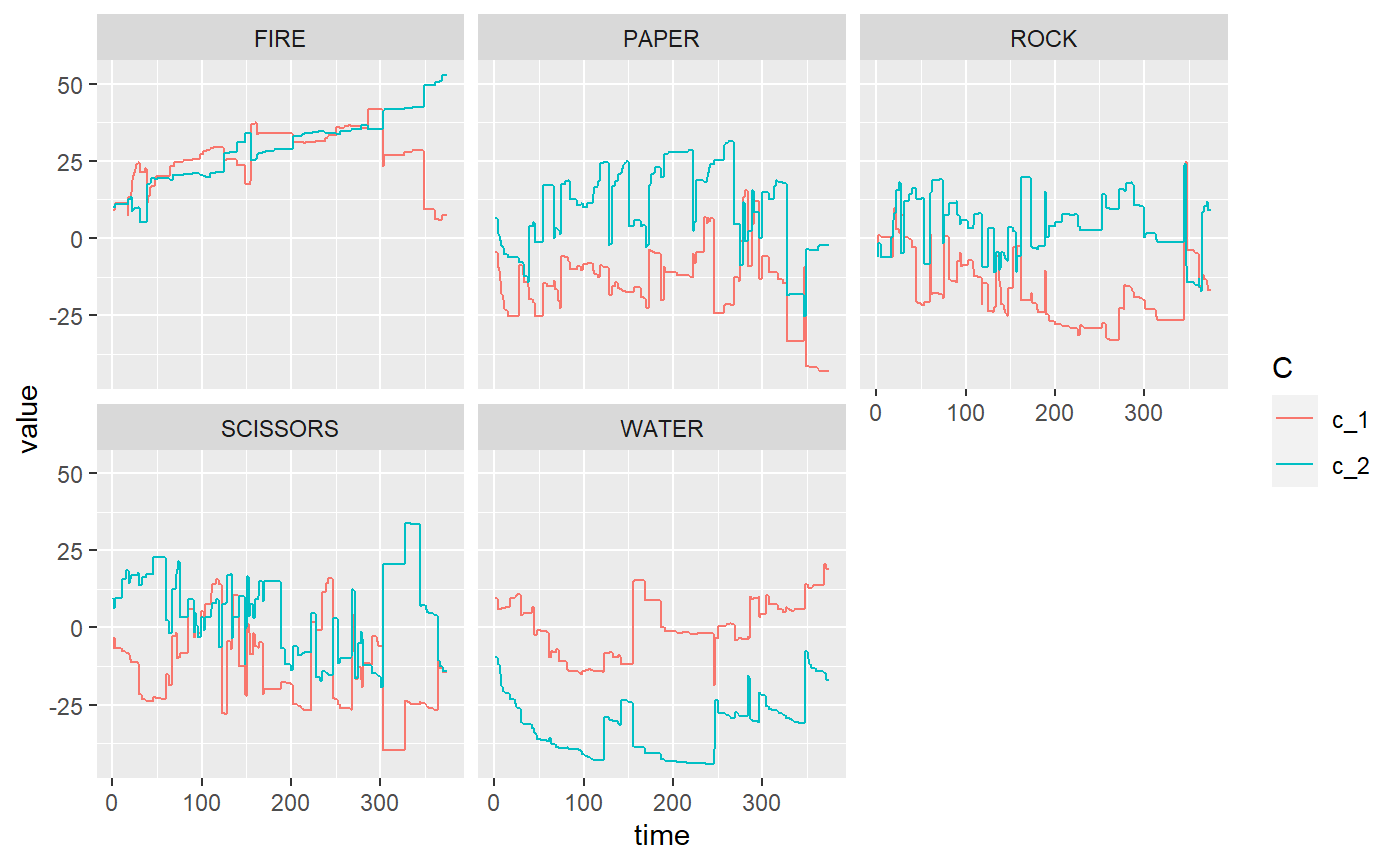
plot_c_mat(rpsfw_mELO_1)

Further playing around with learning rate parameters and the number of training matches fails to improve these results. Let’s fit a mELO model with $k=2$ which should have more capacity to capture the non-transitive dynamics exhibited here.

mELO model with $k=2$

rpsfw_mELO_2 <- mELO(rpsfw_df, k=2)
rpsfw_mELO_2
#> 
#> mELO Ratings For 5 Players Playing 375 Games
#> 
#> k = 2.
#> 
#>     Player Rating Games Win Draw Loss Lag
#> 1     FIRE 2260.1   150  90   30   30   2
#> 2    PAPER 2211.8   150  60   30   60   0
#> 3 SCISSORS 2201.9   150  60   30   60   5
#> 4     ROCK 2170.7   150  60   30   60   3
#> 5    WATER 2155.4   150  30   30   90   1

# Get predictions
rpsfw_mELO_preds_2 <- predict(
    rpsfw_mELO_2,
    rpsfw_sample_df
)

data.frame(
    rpsfw_sample_df,
    mELO_preds = rpsfw_mELO_preds_2 %>% round(3)
)
#>    time_index  throw_1  throw_2 outcome mELO_preds
#> 1           1     FIRE    PAPER       1      0.999
#> 2           2     FIRE     ROCK       1      0.998
#> 3           3     FIRE SCISSORS       1      0.999
#> 4           4    PAPER     ROCK       1      0.998
#> 5           5    PAPER    WATER       1      0.998
#> 6           6     ROCK SCISSORS       1      0.999
#> 7           7     ROCK    WATER       1      0.999
#> 8           8 SCISSORS    PAPER       1      0.998
#> 9           9 SCISSORS    WATER       1      0.999
#> 10         10    WATER     FIRE       1      0.999

# Inspect advantage matrix
get_adv_mat(rpsfw_mELO_2)
#>               FIRE     PAPER      ROCK  SCISSORS     WATER
#> FIRE         0.000  1137.019  1037.469  1078.412 -1275.408
#> PAPER    -1137.019     0.000  1068.633 -1094.378  1057.697
#> ROCK     -1037.469 -1068.633     0.000  1190.589  1174.887
#> SCISSORS -1078.412  1094.378 -1190.589     0.000  1180.526
#> WATER     1275.408 -1057.697 -1174.887 -1180.526     0.000

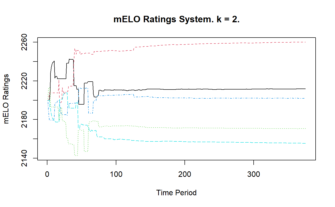
These predictions are spot on and the $\textbf{A}$ matrix is in line with our expectations. Let’s inspect the historical ratings and vectors

plot(rpsfw_mELO_2)

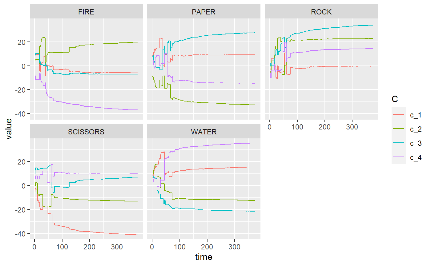
plot_c_mat(rpsfw_mELO_2)

Whilst an ordinary Elo model and mELO model with $k=1$ fails to capture the dynamics rock-paper-scissors-fire-water, a mELO model with $k=2$ succeeds.

Other features

See the help files for details on the other available functions:

These functions can be used for diagnostic purposes or help prepare data for model outputs for custom plots.

Introduction to mELO ratings

David Lazaridis

2020-05-16